Introduction

Today, we’re releasing our cost-effective hyperparameter optimizer, CARBS, which enables researchers to more easily scale small experiments to large models.

As part of our efforts to train a 70B-parameter language model, we conducted extensive experimentation at a smaller scale. There were two goals of the small scale experiments: to choose optimal hyperparameters for the larger scale run, and to predict the performance of the large scale run.

One challenge with small scale experiments is that, due to the noise in the training and language modeling process, it is difficult to compare the performance of two models on benchmarks that are still relevant at a larger scale. This motivated the development of a metric that is both sensitive (giving meaningful results even for models with fewer than 300M parameters) and repeatable (where the same training procedure gives the same result).

Next, we used this metric with CARBS, our cost-aware hyperparameter tuning algorithm, to tune dozens of hyperparameters over thousands of experiments at small scale. While some hyperparameters, such as the data mix, could be kept fixed while scaling from small experiments to large ones, this was not possible with others, such as the learning rate, the number of attention heads, or the multi-layer perceptron (MLP) width. Because CARBS generates optimal values for a range of costs, we could extrapolate from the Pareto set of observations to find how we should scale each parameter as we scale up our training. This allowed us to accurately predict the performance of our final model.

Developing the metric

Evaluations of pre-trained language models have evolved significantly since the early days of transformers. BERT was evaluated by fine-tuning the pre-trained model individually on various text classification tasks. GPT-2 primarily used perplexity measures on different datasets. GPT-3 showed that many of the classification tasks could be completed in-context with zero- or few-shot prompting for larger models, removing the need for additional fine-tuning. These in-context learning (ICL) benchmarks remain popular today for evaluating pre-trained model performance, although the use of supervised fine-tuning and reinforcement learning (RL) methods somewhat muddles the picture when comparing with closed source models. Another option for large language model evaluation is Elo ranking of language model generations, either by humans or a large language model (LLM) judge. We will discuss our own experiences with using these different evaluation metrics with small and large models.

ICL evaluations: completions vs. multiple choice

First, we considered evaluations that could be done without fine-tuning.

Since language models are trained to predict the next token, one natural way to evaluate them is through a task like LAMBADA, where a passage is presented to a language model to see if it accurately predicts the following word. Passages are chosen such that the final word is obvious to human raters.

Single-token completion for LAMBADA. The language model is presented with the context (left), and the next token probabilities are used to score whether the model makes the correct prediction.

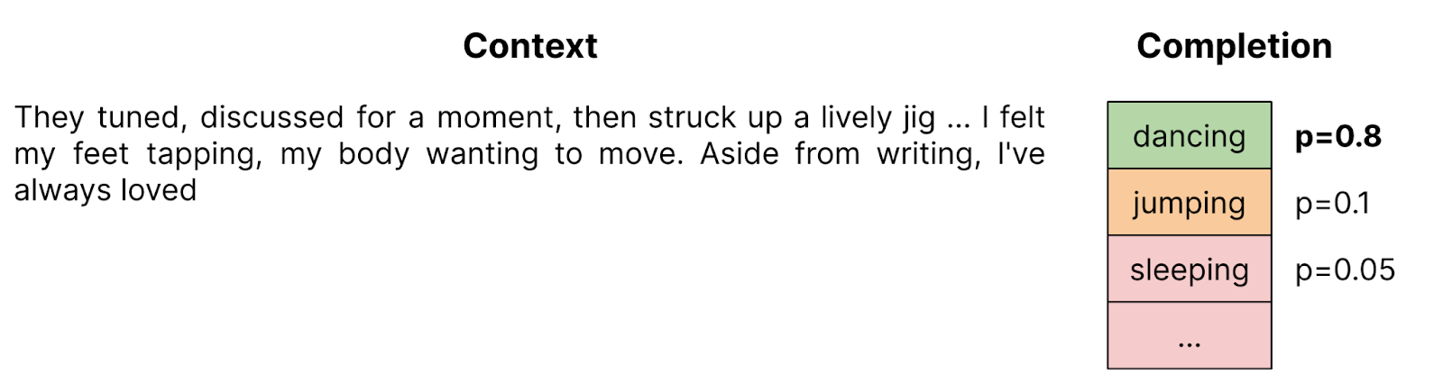
While single-word prediction is a good test of language models in their native format, it does not capture many types of activities we want language models to do. For example, if we want language models to be good at completing a sentence, rather than just finding the next word, we might turn to the HellaSwag dataset, which asks the language model to find the best completion for a sentence among four options. We could naively extend the idea of using word probabilities to compare the probabilities of full sentences by multiplying the probabilities of each word.

Multi-token completion for HellaSwag. The language model scores the probability of each sentence by multiplying the probabilities of each token if placed after the context. If the highest probability is assigned to the correct completion, the language model is judged to give the correct answer.

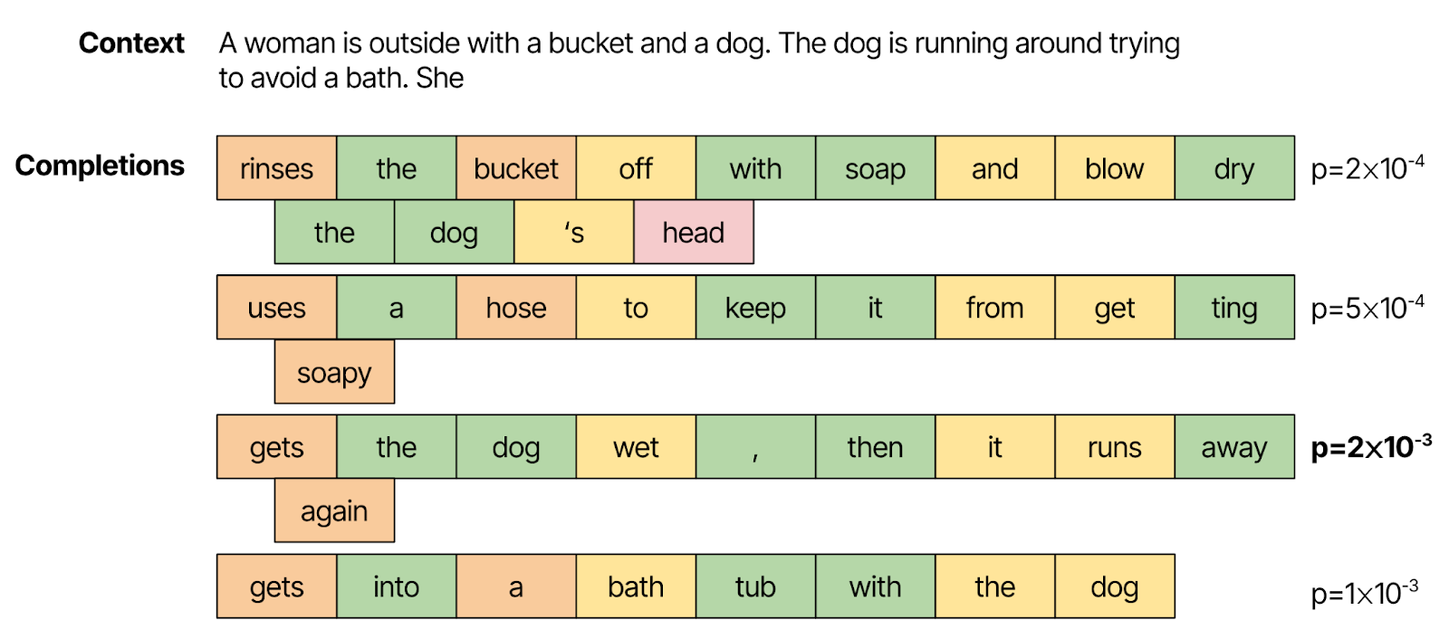
However, this is subject to a few sources of noise and bias. If the “correct” generation makes a single word choice that the language model considers very low probability, it will score that generation lower, even though a similar, grammatical completion might be considered high probability. Longer generations are also penalized with lower probabilities, as more words must be chosen correctly. Normalizing the completion probabilities by answer length is a common workaround, but does not address the fundamental challenges at play here.

One fundamental issue with this formulation is that the language model is not able to see the four possible completions it is choosing from, and therefore cannot express probabilities over them in a meaningful way. One way around this is to present the dataset as a multiple choice question, where the “completion” is the letter of the answer (i.e., A, B, C or D).

HellaSwag as a multiple choice question. Here, the completions are single tokens, so the probabilities make more sense again.

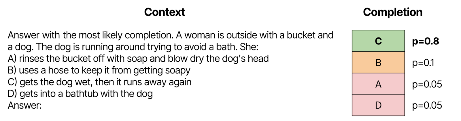
Because the answer comes after all completions, the model can assign probabilities to the answer token with a complete context. Unfortunately, because this format is not typical of the training data, we see that performance of even larger models is fairly poor.

ICL evaluations vs. fine-tuning

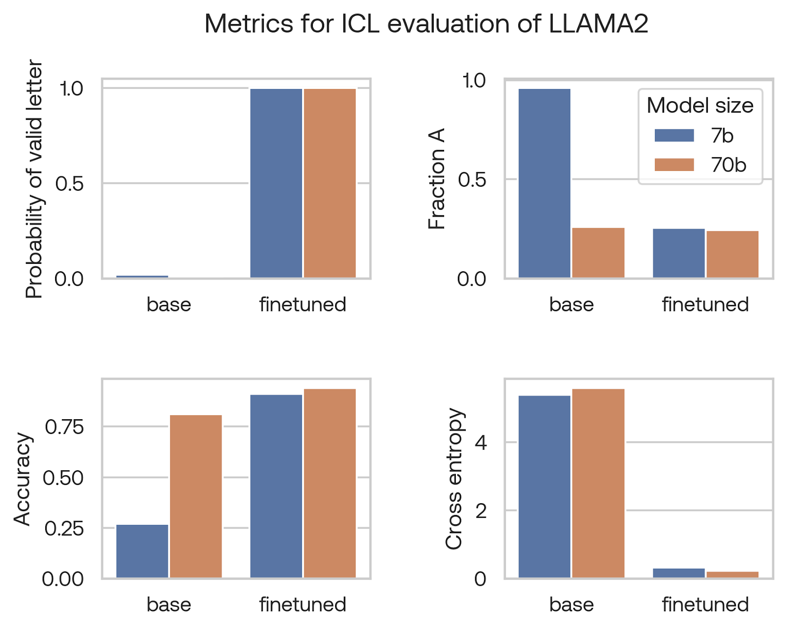
We found that using multiple choice questions is a good way to provide all the necessary context to a language model, allowing it to answer complex questions using simple next-token prediction. However, we found that both small and large language language models put very low probability on any valid answer (see “probability on A/B/C/D” in the image). When forced to choose between the candidate letters, smaller models had a very strong preference for the first answer “A” (see “Fraction A” in the image). We thought this may have to do with our prompting, or the fact that “A” is a word and “B” is not, but this phenomenon occurred even when we randomized the letters and added few-shot prompting.

Comparison of Llama 2 7B and 70B on RACE before and after fine-tuning.

We tried many other techniques, including randomizing the letters, adding tags like [answer]A[/answer], and using pointwise mutual information correction, but were unable to find a metric that would give us a strong signal at the 7B-parameter model scale.

Because of this, without fine-tuning, the Llama 2 7B model we tested had essentially the same performance as a random network. Looking at the cross-entropy was no better: it was far worse than random performance (which would be 1.2 for four choices), and the larger model performed worse than the smaller one.

We realized we would need to fine-tune our pre-trained language models in order to evaluate them. We tried fine-tuning on individual evaluation datasets as well as all the datasets together, and found that the performance was quite similar (see table below).

This allowed us to robustly probe the abilities of the language model. The answers became uniformly distributed over the answer choices and no other tokens, allowing us to trust in the probabilities output by the model. Fine-tuning on the evaluation dataset learned significantly more than the surface form; fine-tuning on a dummy dataset, which contained extremely simple questions and answers, did not perform nearly as well.

Answer cross entropy vs. accuracy vs. perplexity

Once we were able to get consistent results out of smaller language models, we considered how to report and aggregate the results. While accuracy is easier to interpret, the cross-entropy of the correct answer token might give an earlier indication of learning on difficult problems.

If we were using correct answer cross-entropy, why not simply use perplexity on a relevant set of documents? One reason we mentioned earlier is that perplexity can be noisy when the document contains word choices that the model assigns low probabilities. Moreover, measuring perplexity on the full document does not capture the knowledge we are trying to test for with our evaluation tasks. Finally, the perplexity measure ends up being tied to choices of tokenization that we want to evaluate separately.

Why not generative evals?

In the end, we wanted to create language models that do more than just answer multiple choice questions. Why didn’t we include any evaluations of the model generations, either through chain-of-thought prompting to answer questions, or by an LLM judge? For one thing, the <1B models tend to perform quite poorly at generation, so judging which mangled output is better becomes a challenging exercise.

More importantly, we think that the fine-tuning done to improve outputs is a separate process from the pre-training one. If the features of the pre-trained model are better, we believe the generations after fine-tuning and RLHF will be better. This type of single-token fine-tuning is a more direct probe of the features in the pre-trained model, whereas generative evaluations carry significant noise due to the properties of fine-tuning and RL performed on top of the model.

Datasets and weighting

We considered 47 different evaluation datasets on criteria such as dataset size, quality, and relevance to reasoning and coding tasks. The evaluations we chose, with the weights and dataset size, are below. We held out 1,000 of each dataset for validation and 1,000 for the test set, and the rest were used for fine-tuning.

Here are a few notes about relevant datasets:

• CodeComprehension. We created a large dataset of questions about generated Python code, which contains a mix of code evaluation and cloze-style tasks. This dataset is up-weighted significantly as it is the only coding related dataset in our metric. We are releasing the dataset on Hugging Face.
• GSM8K. This dataset presented a challenge for our evaluation metric, as it does not include multiple choice options. To generate wrong but believable answers, we created a pipeline to mutate the math operations that are applied, as well as which numbers from the original problem are used for the operations. Note that we fine-tuned and evaluated on solving this dataset without any chain-of-thought, making this by far the most challenging dataset in our metric.
• ARC: We found these questions to be similar to the ones we are most interested in, and up-weighted it accordingly. We only included the ARC Challenge dataset.
• WinoGrande, HellaSwag, and BoolQ: We found these public datasets to be lower quality and down-weighted them accordingly.
• MMLU: We did not include this dataset, as we found these problems to be too challenging for smaller models to solve in our setting.

Creating proprietary held-out sets

We used the metric described above for all of our validation sets. We also did a significant amount of work to create clean, high quality test sets, which we wrote about here.

Using CARBS to tune and scale LLMs

We developed CARBS to allow us to tune hyperparameters while scaling up deep learning models. CARBS is a cost-aware local Bayesian search algorithm which leverages the fact that optimal hyperparameters tend to vary smoothly as the amount of data and number of parameters in a model increase. This allowed us to conduct many low-cost experiments that directly predict optimal hyperparameter values for high-cost experiments. We’ve previously written an in-depth blog post on how CARBS works. Here, we will go over some of the CARBS experiments we ran at the smaller scale (300M- to 3B-parameter models), and then show how we were able to accurately predict performance when scaling up the model.

Tuning our data mix

Our initial investigation was into optimal data mix for pre-training. We tuned the weighting for 11 different datasets, together with three filtering parameters for our Common Crawl data: a perplexity filter, a spam filter, and a general quality filter. The perplexity filter is based on the KenLM language model. The spam filter and general quality filter use scores based on binary fastText classifiers trained on labeled documents from the source distribution, answering the questions “is this document spam?” and “does this document contain a coherent main body of text?”. Because we wanted an accurate picture of how the data mix and filters would perform when we became data-limited at large scale, we truncated each dataset based on the model size. Consequently, a model with N billion parameters would only see N/100 of the training examples.

We also used three scaling parameters for the model: the number of heads, the number of layers, and MLP hidden dimension. We fixed the head dimension to 128 and included one parameter for the data: the number of tokens used for training. We also tuned both the pre-training and fine-tuning learning rate, together with the training batch size, for a total of 21 tuning parameters.

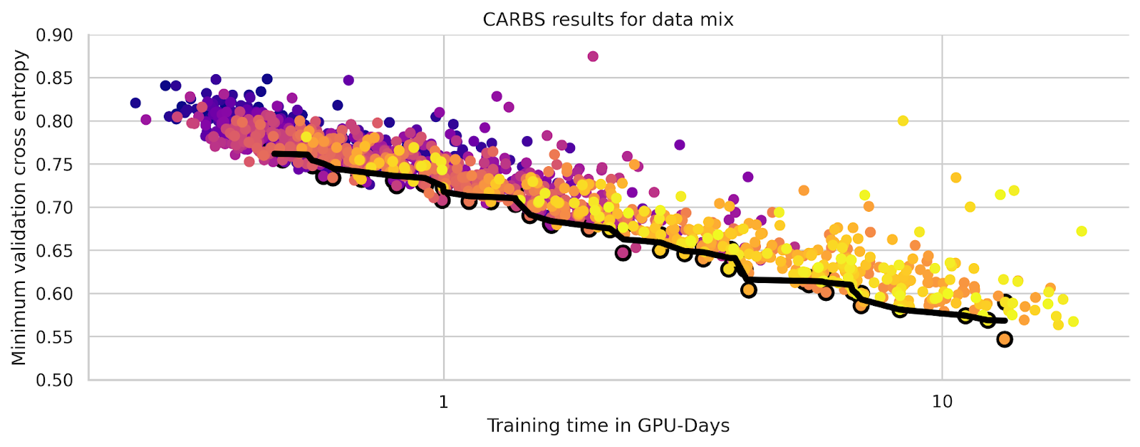
Each experiment was small enough to train on a single node, so we were able to run 80 experiments in parallel. In order to simulate scaling up larger experiments to more nodes, we added a number of gradient accumulation steps proportional to the model size. The graph below shows the resulting Pareto frontier in black, with the Pareto efficient points outlined in black. The color of each point indicates the order in which CARBS ran each experiment: starting from purple, transitioning to magenta, and concluding with the most recent runs in yellow.

Minimum validation cross entropy after pretraining various models with hyperparameters selected by CARBS. Each point represents a pretraining experiment, with over 1400 experiments run. The points with a black border are on the pareto front. The lighter color points are collected by CARBS later in training. The pareto front shows consistent scaling of the model.

The results for each data parameter are shown below. In these plots, each point is an experiment, with the y-axis indicating one search variable and the x-axis indicating the amount of time the experiment took to run. The color of the points indicates the fine-tuned cross-entropy on our evaluation set. The Pareto set of points are again outlined in black. A dashed black line is fit to the Pareto set. The colored lines indicate curves of constant performance according to the underlying Gaussian process model. For the datasets weights, the weight is relative to Common Crawl data, so a value of one would be one epoch of the dataset per one epoch of Common Crawl.

Individual parameter plots for each data mix experiment run by CARBS. Each data point represents a complete pretraining experiment. The color of the point indicates the validation cross entropy after fine tuning the experiment. The curved lines show predictions from the gaussian process model used by CARBS when varying the parameter shown on the y axis. The points outlined in black are on the pareto front, and the black dashed lines are a linear fit to those points.

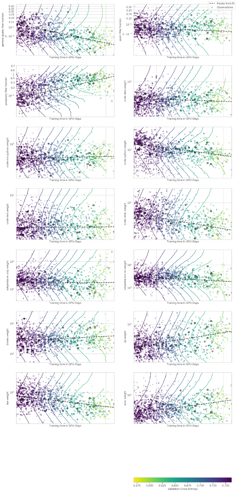
Here are a few conclusions from these experiments:

• The quality and spam filters did not seem to be useful. However, the perplexity filter seems to be very helpful, more so for experiments in the middle of this cost range. Ablation experiments at a larger scale found that this filter was not helpful for improving performance, so this may have been a case of the tuning finding a spurious correlation here.
• Non-Python code did not seem to improve performance significantly. Python code seemed to be only about as good as the Common Crawl data, despite Python questions composing about 40% of our evaluation weight.
• Books and Wikipedia appeared to be by far the most valuable data. Surprisingly, non-English Wikipedia was as helpful or slightly more helpful than English Wikipedia.
• Other structured, high quality data did not seem to shine in this setting. StackExchange (labeled QA for question answering in the plots above), Law, and arXiv were mixed in at slightly lower rates than Common Crawl. These datasets may be too complex for these smaller models to fully make use of.

Scaling experiments

With our data mix chosen, we performed another set of experiments with fixed parameters, which focused on reaching larger scale models. For these experiments, we scaled up the number of nodes used for an experiment proportional to the model size, so that we would find hyperparameters allowing us to use our full cluster for the larger run.

Because CARBS uses the amount of time a run takes to estimate how well it did compared to other runs, it was important to have consistent InfiniBand performance for runs across our cluster. See some of the work we did to ensure consistent performance in our other blog post.

We used seven total tuning parameters: the three model size parameters, number of tokens, two learning rates, and batch size. Because the runs occupied a varying number of nodes, we were able to run about 30 different experiments in parallel.

Minimum validation cross entropy after pretraining various models with scaling hyperparameters selected by CARBS. Each point represents a pretraining experiment, with over 400 experiments run. The points with a black border are on the pareto front. The lighter color points are collected by CARBS later in training. The pareto front shows consistent scaling of the model.

Individual parameter plots for each scaling experiment run by CARBS. Each data point represents a complete pretraining experiment. The color of the point indicates the validation cross entropy after fine tuning the experiment. The curved lines show predictions from the gaussian process model used by CARBS when varying the parameter shown on the y axis. The points outlined in black are on the pareto front, and the black dashed lines are a linear fit to those points.

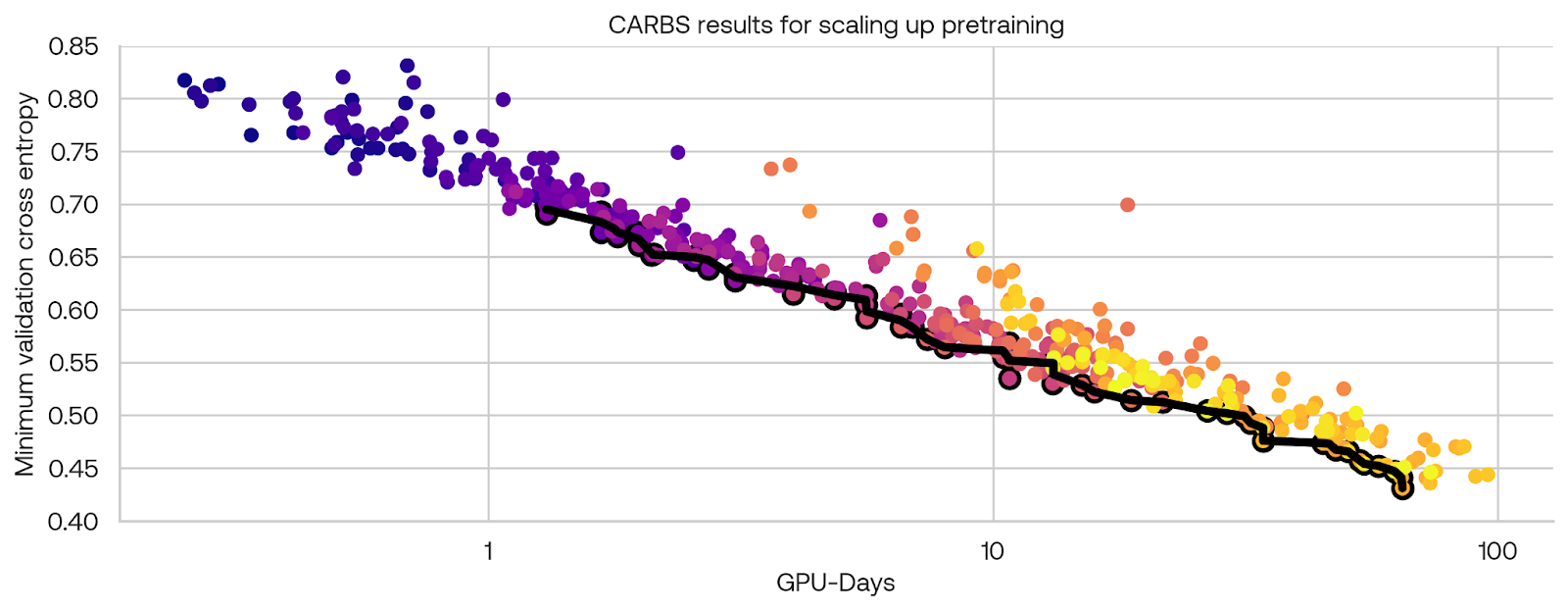
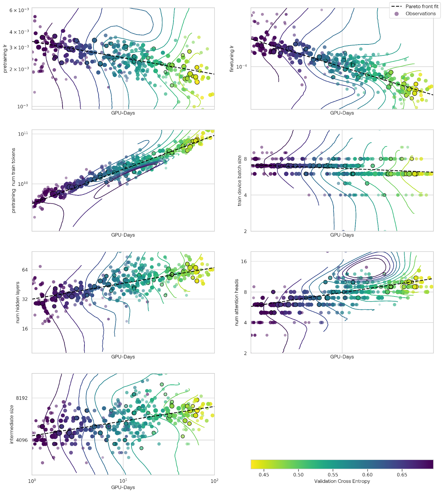
These plots demonstrate an unusual feature: it looks like there is a cluster of runs at a larger scale (higher cost) that had loss spikes, leading to poor performance. By looking at the parameter-wise predictions, we can determine that this poor performance could likely be attributed to to the model width, rather than learning rate.

It is interesting that the model has converged to narrower, deeper networks than are typical for this number of parameters. This is consistent with previous work suggesting that narrow deep networks have better fine-tuning performance, for the same loss, than shallow wide networks.

Tokens per parameter for the scaling experiments, with the Pareto set fit shown as black dashed line. While the average value is close to the Chinchilla “rule of thumb” of 20 tokens/parameter, the positive slope hints that large models may need to be trained on many more parameters to be compute optimal under our assumptions.

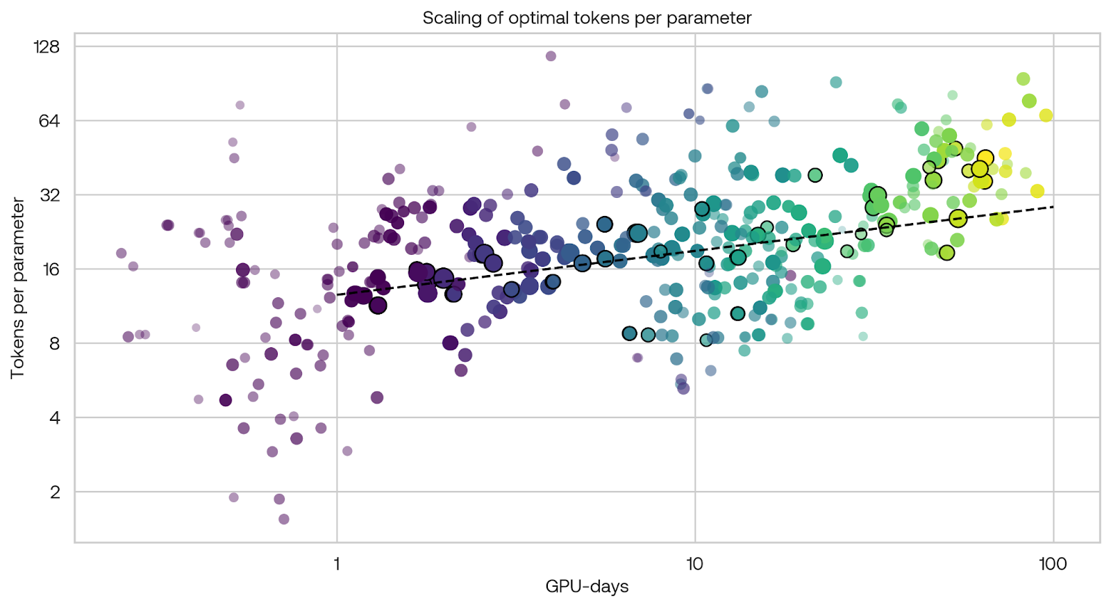
Another interesting finding is the optimal number of tokens per parameter. We found this optimal number to be slightly increasing across our range of experiments (see the dashed black line). Note that our methodology differed from that of Chinchilla in a few significant ways: we explicitly scaled the number of machines together with the model size, effectively changing the batch size. We also measured fine-tuning performance, not training loss. Although we have a significant range of costs in our data, Chinchilla trained relatively more models at higher parameter counts (up to 10B parameters). We consider this set of experiments to be a weak signal, but it certainly seems worth investigating further.

7B- and 70B-parameter experiments

Our goal was to train a model at the same scale as Llama 2 70B. Therefore, we targeted both 70B parameters and 2T tokens. On the way to this full scale experiment, we opted to train a 7B-parameter model on 200B tokens. We used the above scaling experiments to update some of the parameters from Llama — notably going to deeper narrower networks and increasing the learning rate.

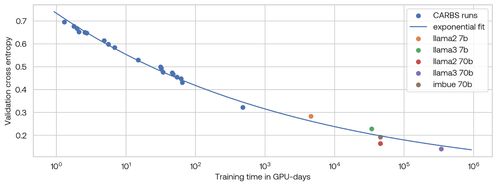
When we plot the performance of our 7B run together with the performance of experiments from our CARBS run that were near the Pareto fit line, versus the amount of compute used for training, we find that an exponential fit accurately predicts the performance of the 70B parameter model that we trained.

A power law fit of CARBS experiment performance versus training time extrapolates well to the performance of our final 70b parameter run.

Further fine-tuning

In all the above experiments we used the same fine-tuning parameters, except for the learning rate. We found that by reducing the batch size and running CARBS again on the fine-tuning hyperparameters, we could improve the performance on our metric from 0.192 to 0.169:

Minimum validation cross entropy when fine tuning the imbue 70b model. Each point represents a fine tuning experiment, and the black points are on the pareto front. The performance starts to get worse after around 1.5 epochs.

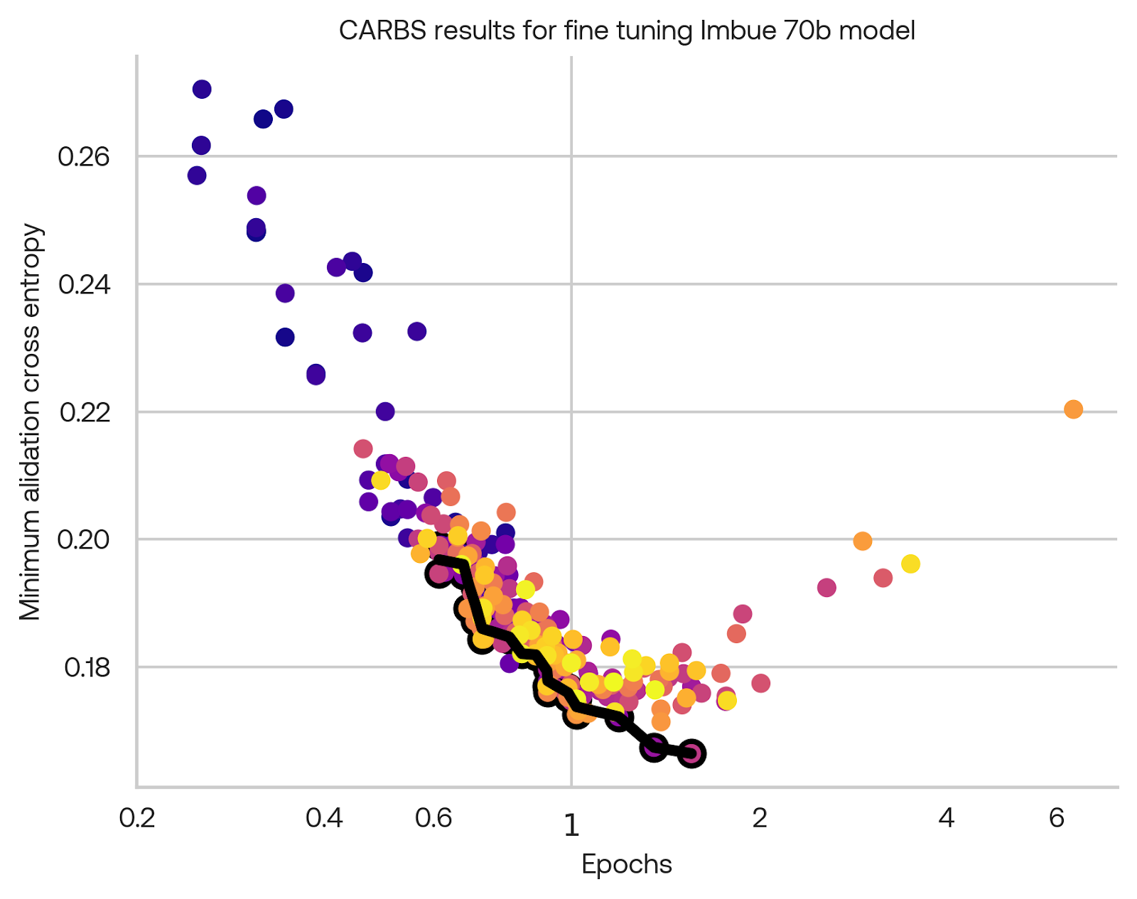
The optimal fine-tuning configuration was to do one epoch over the fine-tuning data. More epochs actually harmed performance: at the one epoch point, performance would be worse if the overall training epochs were longer. This indicates the learning rate schedule (a cosine decay over training) is important for getting the most out of fine-tuning data.

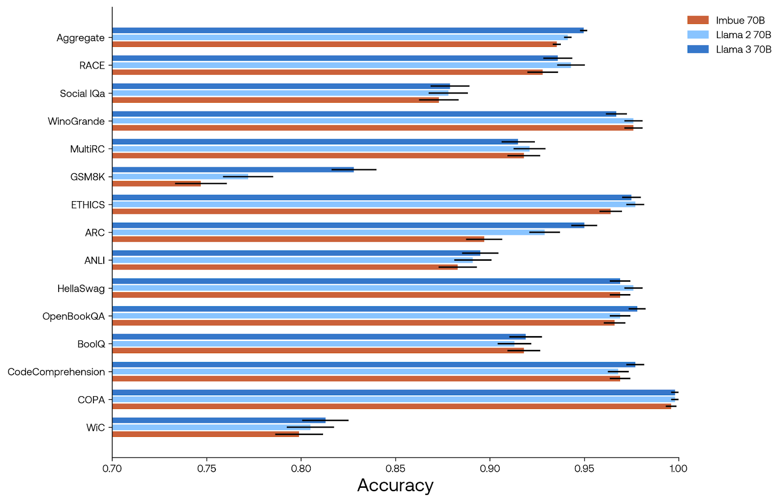
The performance of the fine-tuned Imbue 70B model is roughly similar to Llama 2 70B on most of our evaluation datasets, although aggregated performance is worse. This can mostly be attributed to a few difficult tasks (GSM8K and ARC) that may benefit from seeing significantly more domain specific data in pre-training. See our evals blog post for a more thorough analysis of the Imbue model performance compared to other models.

Performance of our fine tuned 70b model on various datasets used in our CARBS metric.

Conclusion

Training a large scale model requires making many hyperparameter choices, from data weights and filtering parameters to network size parameters and learning rate schedules. In order to enable small scale experimentation, we developed a sensitive metric that allows us to reliably make comparisons between small language models (<1B parameters) using the same evaluation metric that applies to large scale models. This means that we can do many more experiments to find optimal hyperparameters for the exact same training data and evaluation target we will use at large scale.

We combined this metric with our cost aware hyperparameter optimizer, CARBS, in order to predict how optimal hyperparameters change as models scale. We found a number of unexpected results along the way — for example, an upward trend in the number of tokens per parameter — that may warrant further investigation. Extrapolation from our small scale experiments accurately predicted the performance of our 70B-parameter training.

Because of the huge cost of training modern LLMs, researchers are typically conservative when choosing hyperparameters, staying close to previously established values. By releasing the details about our metric and our CARBS optimizer, we hope that others will be able to explore parameter space more fully. We hope this can also be a boon to scaling novel architectures, where working hyperparameters for large models may not be known at all.