A PyTorch implementation of SIMONe

Summary

We recently reproduced and published a PyTorch implementation of the paper SIMONe: View-Invariant, Temporally-Abstracted Object Representations via Unsupervised Video Decomposition. This post walks through the code and provides a detailed explanation of the architecture they use in order to perform object segmentation on videos in a fully self-supervised manner.

Motivation

SIMONe is an approach to the problem of unsupervised visual scene understanding - in other words, learning to compress a high-dimensional raw input (millions of pixels in a video) into a useful low-dimensional representation (some small number of numbers that say something about how many objects are in the scene, what shape they are, how they move, etc). This is a specific version of the more general problem of unsupervised representation learning, where techniques like autoencoders and contrastive learning are commonly used to compress anything (ex: video, images, audio, etc) to a smaller, more meaningful representation.

Intuitively, a good scene representation would probably separate different objects from each other. However, creating supervised data about exactly what constitutes one object vs another is tricky, time-consuming, and ill-defined. What if we could get a network to learn this kind of understanding all on its own? That’s exactly what SIMONe does!

Just from unlabeled, normal video, SIMONe can create segmentations like this:

SIMONe segmentations

Such segmentations seem to indicate that SIMONe is learning some useful representations of the scene that align with at least some of our intuitions about what might make a “good” representation. Such representations seem like they might be useful for all sorts of downstream tasks, from robotics and self-driving to making agents that have a better understanding of the world.

So how does SIMONe manage to create these segmentations without requiring any annotations from people? That’s what we’ll dive into in the rest of this blog post!

Overview

High level SIMONe architecture

At a high level, SIMONe is a Variational Auto Encoder (VAE). This is what a standard VAE for images looks like:

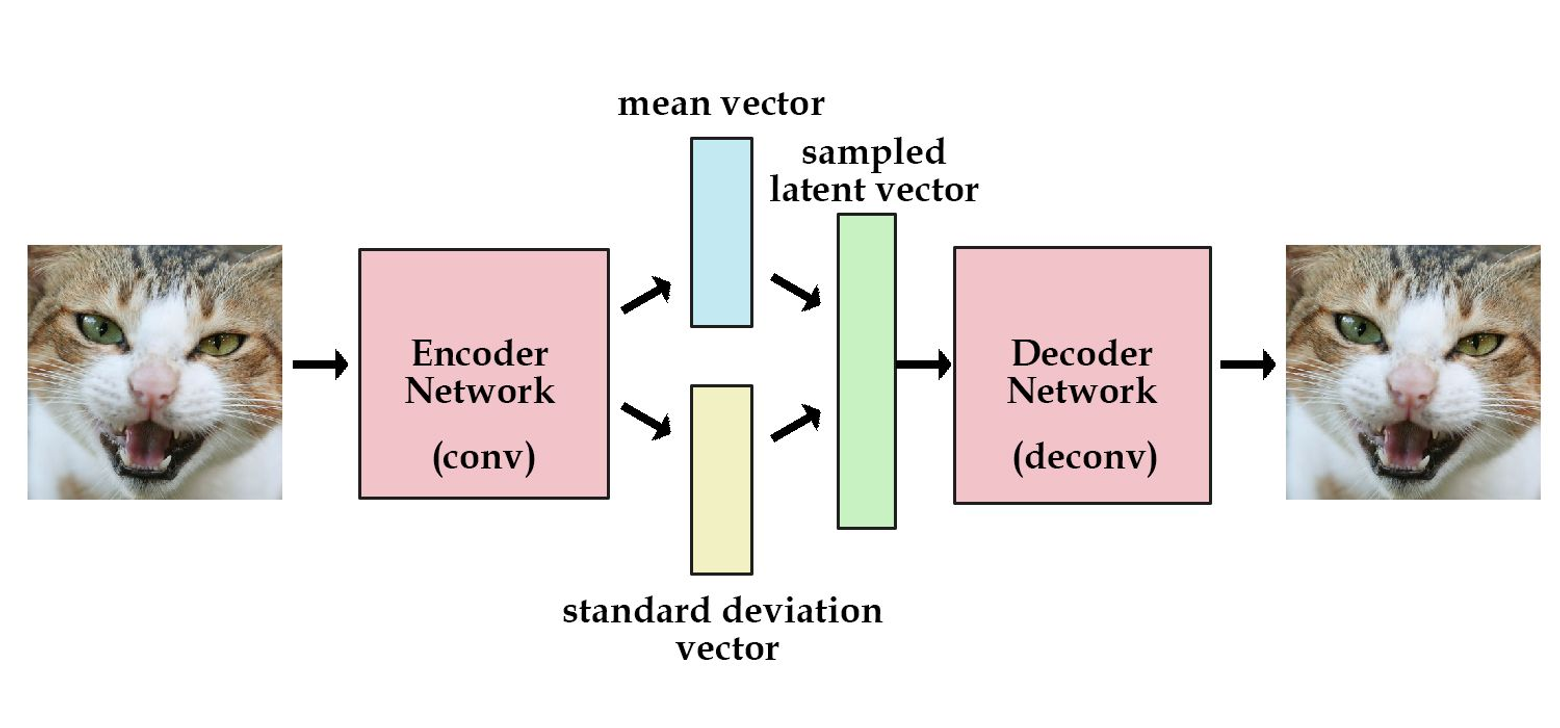
Roughly, a VAE works by taking an input (an image in this example), using the encoder network to create a very small representation of the image, and then using the decoder to expand that small representation back into a whole image. This forces the network to keep only the most important information about the image in that small, middle representation (called the latent), and throw away the rest. Technically, the “variational” part of VAE refers to the exact structure of that latent—it specifies a method of adding noise to the latent, which helps prevent the network overfitting (eg, we don’t want the network to memorize the index of the training example; we want it to store information that applies to any image).

If you’d like to learn more about VAEs and related models, check out this overview of different types of auto encoders.

Slightly more detailed SIMONe architecture

If the above diagram is a standard VAE, this is closer to what SIMONe actually looks like:

Recipe: take one standard VAE, replace input with video, replace output with prediction for a single pixel, add a fancy transformer encoder, split apart the latent, and voila — SIMONe.

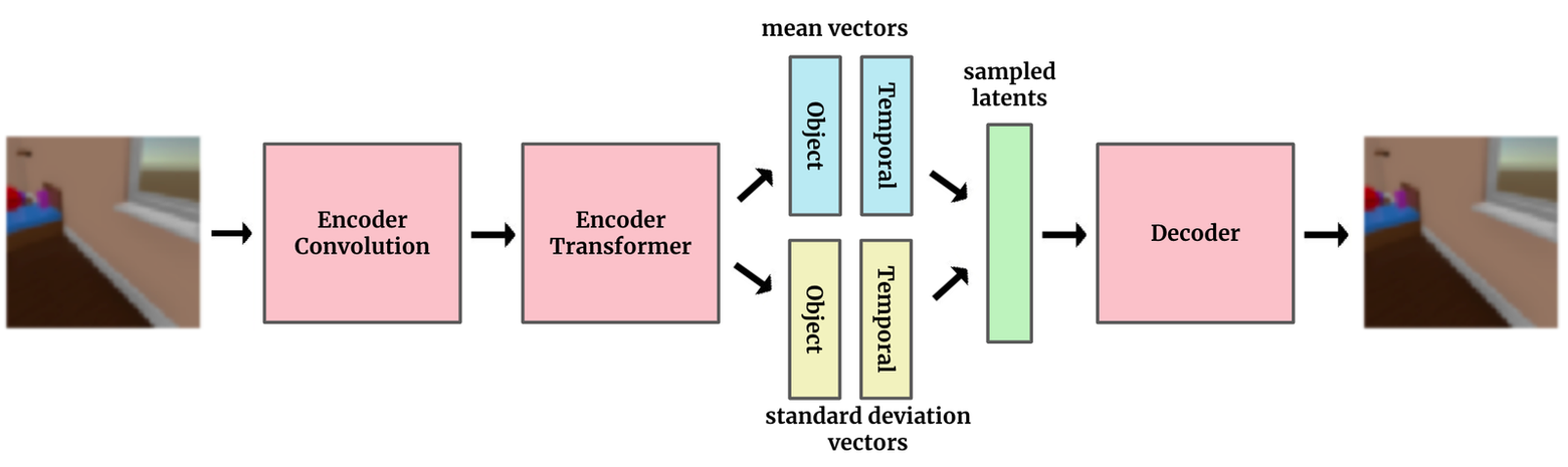
The biggest difference, and the key idea of SIMONe, is to explicitly split the latent space into two separate pieces—one that contains attributes related to the whole video and vary with time, and other attributes that vary per-object.

In the types of datasets explored here, the object attributes encode properties of objects in the scene, like shape, color, and object trajectories, and the temporal, video-level attributes encode things like camera motion. By explicitly architecting the model with this latent structure, we’re hoping to get a representation that gets closer to our intuitive idea of a “good” representation.

The full SIMONe architecture

Below is a full detailed view of SIMONe’s architecture (slightly modified from the one in the paper to be a bit more explicit).

Encoder architecture. Shows the encoding of an entire video into object and frame latents.

Decoder architecture. Unlike a standard VAE, this model predicts each pixel separately. Shows decoding a single frame of the video.

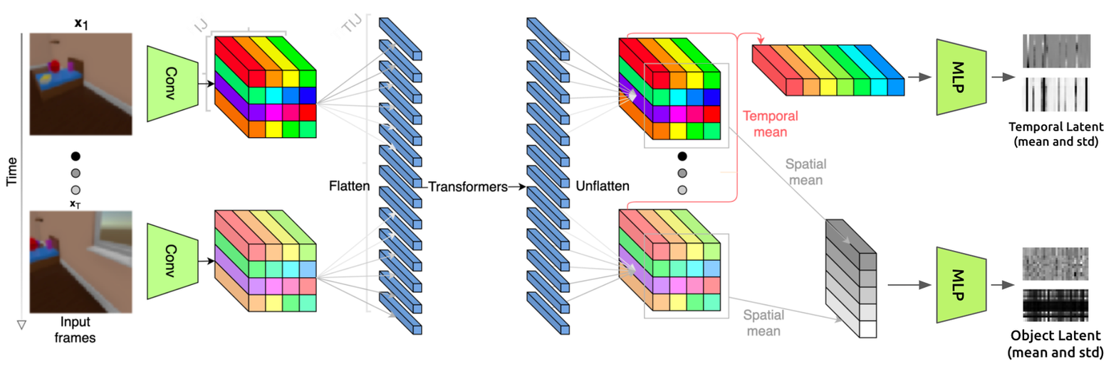
Let’s trace through the entire thing for a quick overview of the model.

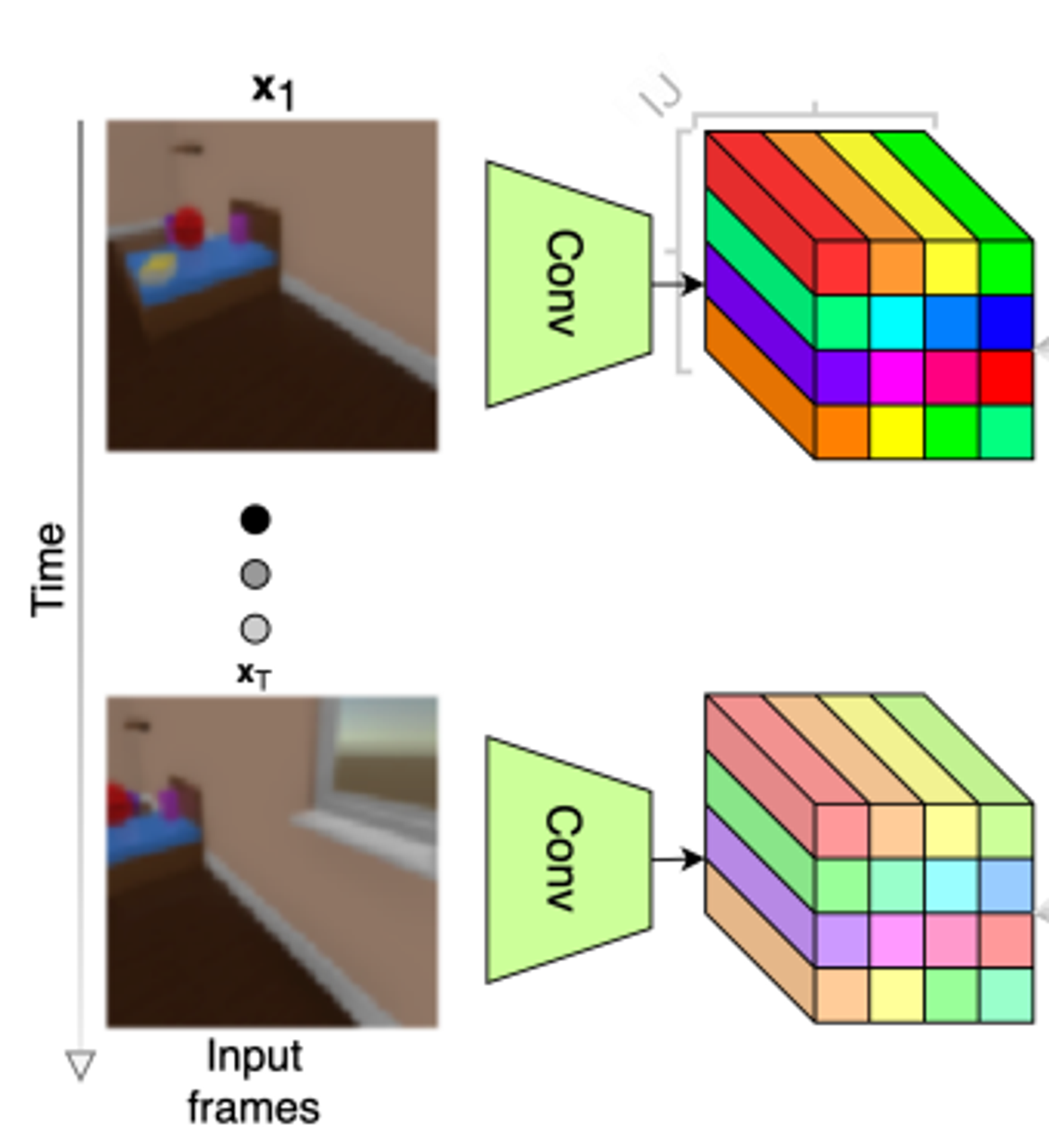
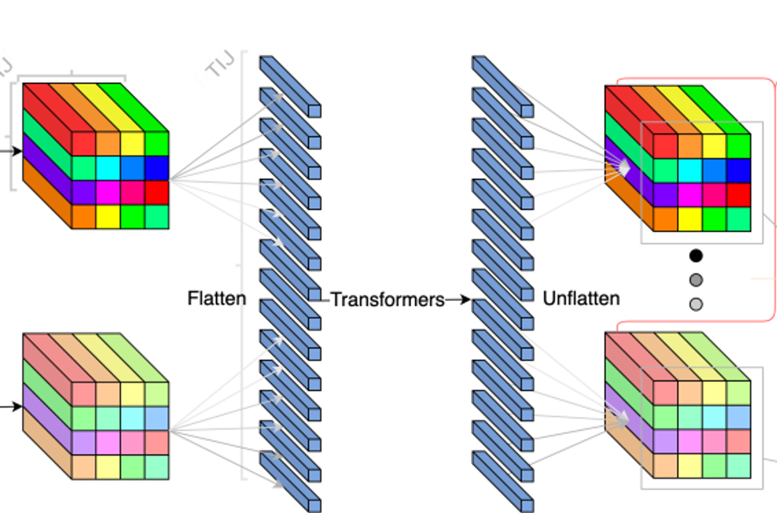
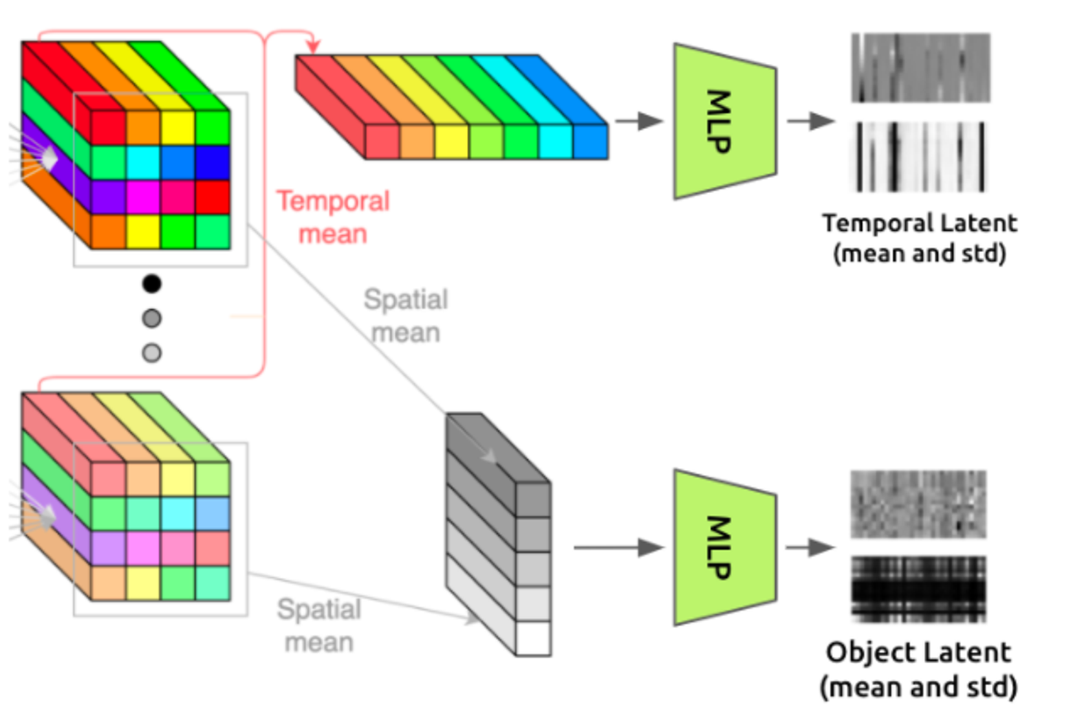
In the first image, We can see that the network input is a series of images (ie, a video). Each image goes through the same convolutional encoder (green trapezoid) to produce an I x J (shown as 4 x 4) grid of tensors representing that image. Those tensors are then flattened, and the resulting sequence is passed through the transformer encoder. The output of the transformer encoder is then grouped back into grids for each frame, then pooled in two different ways (spatially and temporally), resulting in the temporal and object latents, respectively (shown at the right edge of the first image).

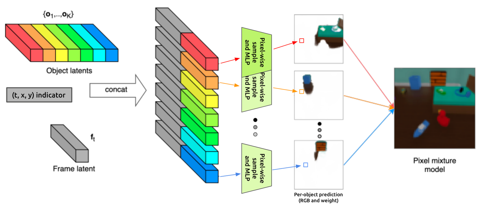
In the second image, we can see those latents as they are concatenated together and passed into the decoder. This is a “gaussian mixture model” decoder, which means that each pixel is predicted independently. In fact, SIMONe predicts K (16) different values for each pixel (one for each object), then creates the final output video as a weighted average of these different predictions. This setup allows for some fancy training tricks (like only reconstructing some subset of the pixels during each training step), though ultimately, the goal is still to faithfully reconstruct the input.

Don’t worry if it’s not clear what’s going on in those images yet—next we’ll walk through each of the 4 major pieces (the 2 encoders, the latent, and the decoder) in detail and show how they can be implemented using PyTorch.

Part 1: Encoder Convolution

First, we need to extract relevant features from the input and compress it into a reasonable size for the transformer. This is accomplished by applying a 3-layer 2D convolution to the input.

python

This corresponds to the first part of the architecture diagram:

Part 2: Encoder Transformer

The second step of the encoder is to apply a transformer to the output of the convolution. While convolutions are good at computations involving local information, transformers are much better at integrating far-away information. This allows each pixel in the output to be influenced by every pixel in the input.

Here, we use a 3d position encoding, which allows the transformer to view the input as a video of 3D shape (t, h, w), rather than a 1D sequence (as transformers were originally designed for),

python

This corresponds to the second part of the architecture diagram:

Part 3: Encoder MLP

Remember that the key contribution of this paper was the unique latent structure. Here’s where we’ll create that structure.

To create a set of constant latents each hopefully representing an “object” in the scene, we’ll take the output of the transformer, which has shape (t, h, w, c), and average it over the time axis to remove the time dependence. This results in a set of “object latent” vectors, each constructed from one of the (h, w) spatial positions.

To create a single set of time-varying latent vectors, we do the same thing but average over the spatial axes. This leaves us with a set of “temporal latent” vectors, each representing one of the timesteps in the video.

The feature MLP performs further computations on these latents by applying a small MLP (with separate weights for spatial vs temporal) to each of the feature vectors in the spatial and temporal latents.

python

This corresponds to the third part of the architecture diagram:

Part 4: Decoder

The decoder makes a prediction of what the input image looked like by using samples from the object and temporal latents. Here’s the decoder architecture diagram again for reference:

At a high level, we’re going to create K RGB videos with per-pixel weights (where K=16 is the number of different object latents). We’re going to do this by drawing an independent sample from the latent for each pixel in that output, adding some indicator (x,y,t) values to that sample, then passing it through an MLP to get the RGB value and weight. After we have these K weighted RGB videos, we’re going to take the weighted average over each of the K values of each pixel to produce a single final video.

It’s rather involved, so we’ve added some extra comments in the forward() function below:

python

That’s the whole model! Now let’s take a look at the loss function.

Loss Function

The loss function is roughly a standard VAE loss function, which has two components:

The first part of the loss is a log-likelihood between the prediction and target video. This is the primary objective—making sure the model is accurately able to reproduce the output. The specific formulation here is a bit unusual—the log likelihood is based not on the final weighted pixels (as is normal), but on a weighted average of the probabilities of each object’s predictions.

python

The other part of the loss function is the KL divergence between the object and temporal latents and their priors (spherical standard normal distributions). This can be viewed as a form of regularization that helps prevent over-fitting.

python

And there we have it! There’s plenty more code required to load in the dataset, run the training loop, monitor progress, compute evaluation metrics, etc., but we’ve covered the most interesting and novel parts of the implementation.

Visualizations

To make the whole process even more concrete, let’s walk through the model again, showing the model outputs at each stage.

We start out with an input video. In our reproduction we used the CATER dataset, one of the three datasets tested in the paper. It has a few static or moving objects in a scene with a moving camera:

After passing through the encoder part of the network, we get object and temporal latent distributions.

Object latent mean. Each horizontal row is the vector representing a single object.

Object latent standard deviation. Black = std of 0, implying that the latent information is important to the decoder.

Temporal latent means. Each horizontal row corresponds to one timestep; time flows downward in the image.

Temporal latent standard deviations. Again, black=0, meaning that darker cells are more important to the decoder.

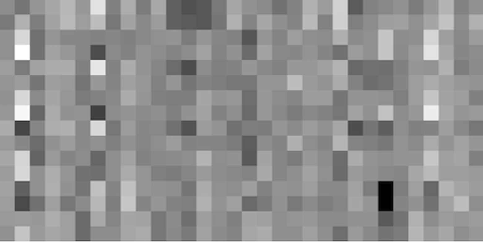
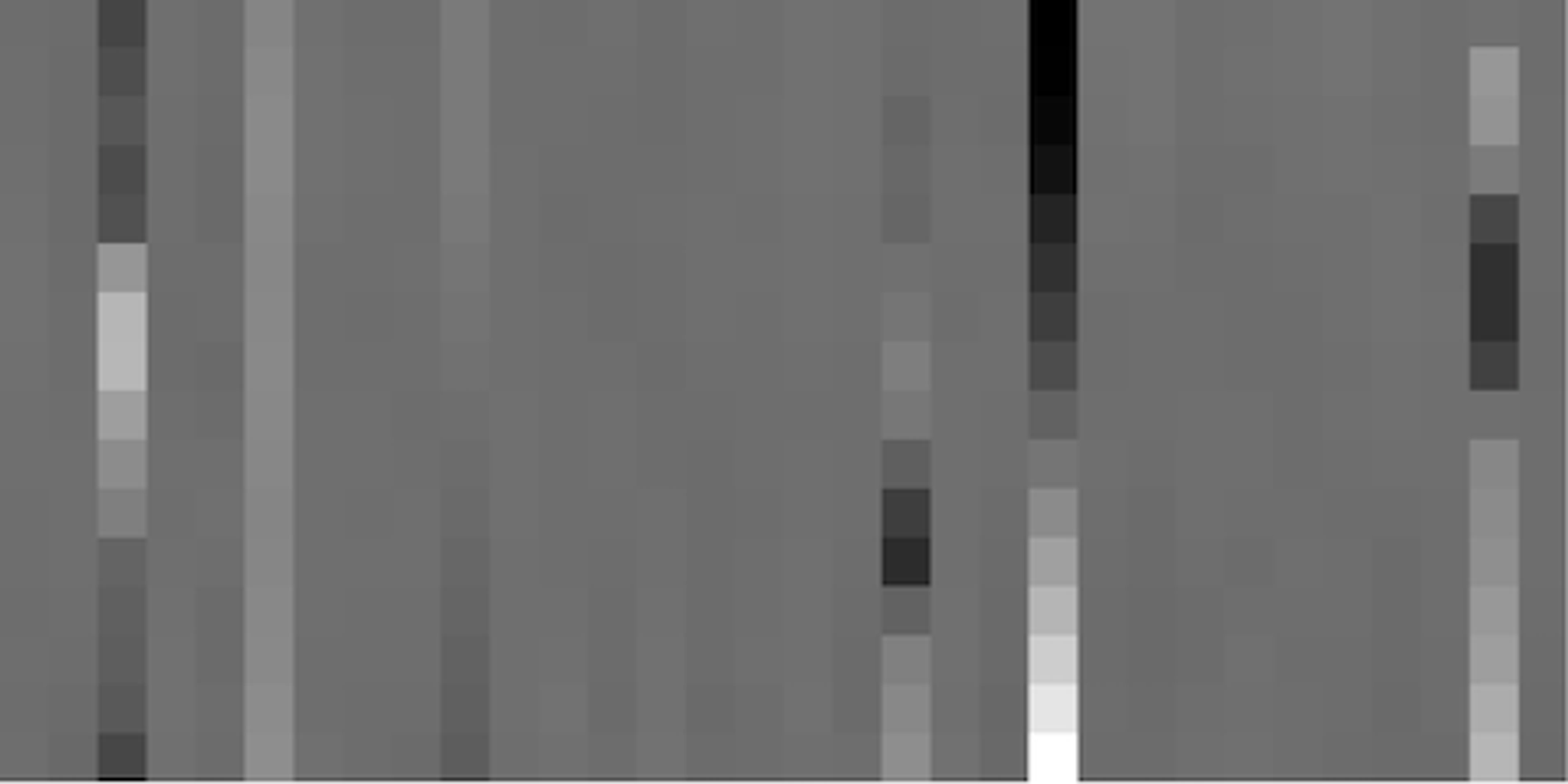
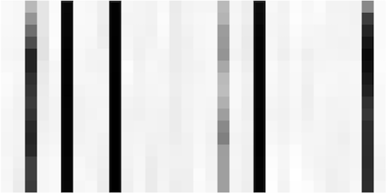
From inspecting the latents, we can observe, for example, that there are about 6 temporal latents that are important for this video (ie, the 6 columns in the last figure that are not very white). The means of those columns (shown in the second to last image) appear to vary relatively smoothly over time (ie, as you look from top to bottom of a column), and they likely represent camera positions, or time.

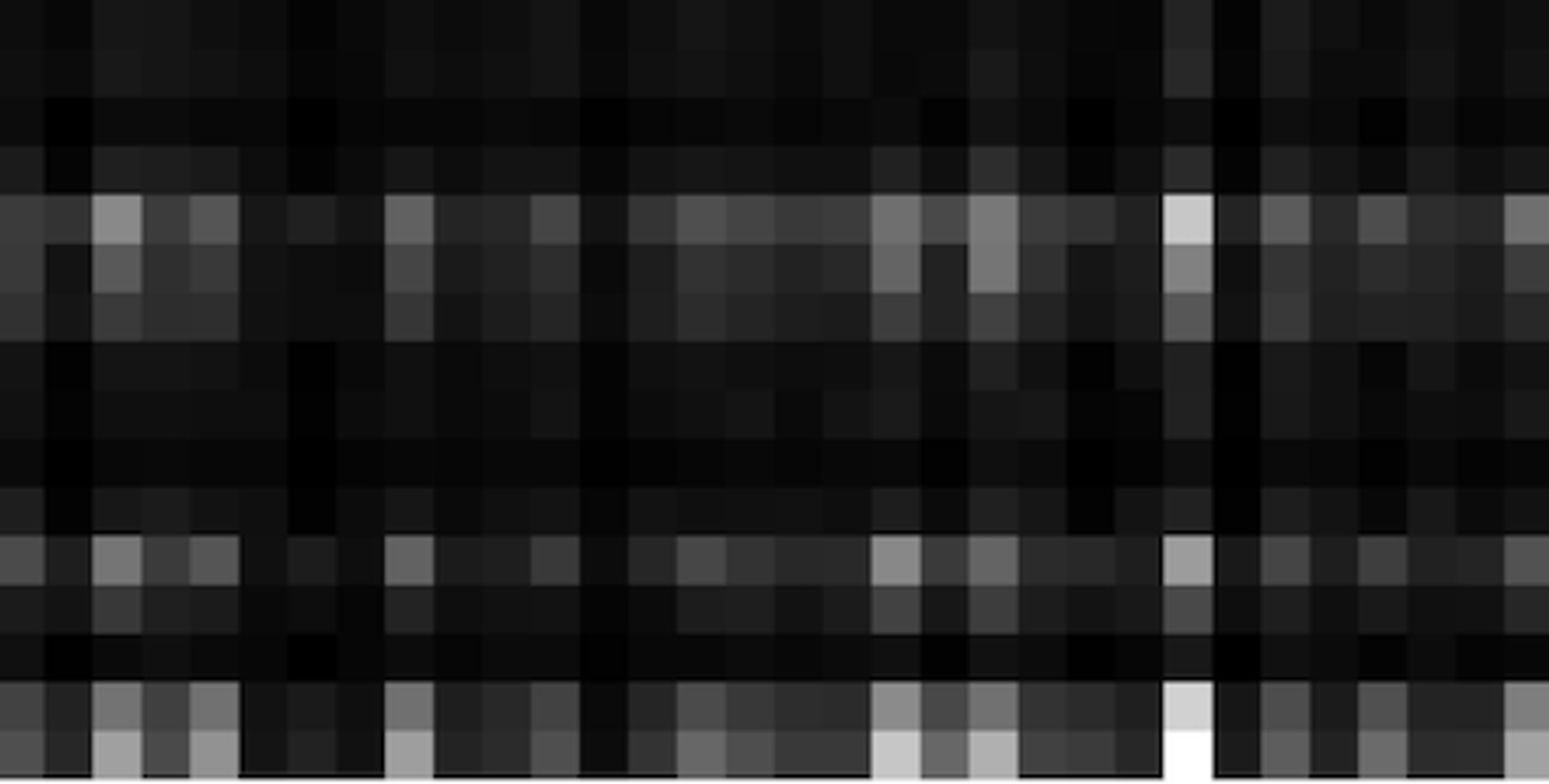
The next step in the process is to put these latents through the decoder, which gives us predicted videos for each of the 16 potential objects:

For a single batch element, the RGB predictions for each of the 16 object latents.

We also get (softmax) weights for each of the 16 objects:

From these, we can construct the final weighted average prediction:

And we can also generate a segmentation visualization:

Our segmentation images don’t look quite as pretty as the ones shown above, but they do have some very clear structure. Our final performance metrics roughly line up with those reported by the authors, so either the final segmentations just normally look like this, or our model ended up doing something slightly different with the background texture that nets a similar final score.

We log extremely detailed training metrics and visualizations for each training run. You can check out an example of these metrics here. Logging detailed metrics was super helpful for understanding what’s going on inside the model.

What next

If you found this interesting, you might enjoy reading the original paper and playing with our implementation.

As always, we’re hiring! You can see our open roles or email us directly at jobs@imbue.com